NoteFun: music and continuous modulation, a tutorial
Written by Michiel Borkent in collaboration with Peter Desain
Introduction
This tutorial provides information about the usage of NoteFun.
This system is implemented in Lisp. We have tried to reduce the amount
of programming-related issues in this article, although all the things
you know about Lisp programming will probably make you a better
composer in NoteFun.
To read more about the workings and implementation of NoteFun, I would like to redirect you to my internship report or the website about my work related to MMM (my internship and final thesis project)
Tutorial
Discrete musical events
In electronical composition one needs to specify elementary musical
events which together constitute a musical piece. The most elementary
musical events in NoteFun are a note and a pause.
For example, (note :pitch 58 :duration .5) and (pause 1.5) are valid events in NoteFun.
The default pitch and duration of a note are 60 and 1 respectively. This means that you can write (note) instead of the longer (note :duration 1 :pitch 60).
As
you can see, the order of the attributes which you specify does not
matter. This is because each attribute goes along with a keyword,
indicated by a colon as the first character. In fact, note
has a lot more attributes which we will ignore for now, as we can use
their default values for the moment. The number which indicates the
pitch corresponds to semitones, whereas the middle-C is indicated by
60.
In composition, like the word indicates itself, we constitute a work
out of more basic objects than the work itself. In our case this means
that we would want to make groups of notes that are somehow related. In
NoteFun
you can make a group of notes in two ways. One way is to make a
sequence of notes and pauses. For example, we could think of the first
line of Are you sleeping (in dutch this song is known as Vader Jacob) as a time-wise sequence of the notes c,d,e and again c. In NoteFun we could compose this as
seq can take any number of notes and groups of notes. For example, we could repeat the first line of Are you sleeping twice, just like in the song itself:
You already can see right now that composition of the complete version of Are you sleeping
would result in a long and unreadable list of 'seqs' and 'notes'. This
problem can be overcome by making a reference to an expression. For
example, we could name the first line of our song line1. This is done by the following:
Now we can represent the double repetition of line1 as:
(seq line1 line1)
which of course looks a lot cleaner.
The second way of grouping notes is ordering them parallel in time. This can be done with sim which stands for simultaneous. For example a major-C triad can be written as
With play we send our composition to a connected midi-synthesizer which then interprets it into sounds. If play is somewhat problematic in your set-up, you might want to use save
instead, which lets you save the musical data as a standard midi file
which you can later use in whatever manner you like. To hear the
example above, listen to this sample:
As you can hear, the melody and the chords get a bit in each others way. It would be nice if we could transpose line1-arrang one octave lower. No problem. We do it with the following construction:
trans takes a number (to be more general, trans takes not only a number but also a GTF)
and a musical object which is decreased or increased in pitch,
according to the number. The number represents a number of semitones as
you might have guessed. -12 then indicates "one octave lower". To hear
the example above click here:
The standard program number (which indicates an
instrument in the General Midi scheme) of a note is 80. It would be
nice if we could use one instrument for melody and a different one for
the rest of the arrangement. Let us change ays in that we
have piano for the melody and strings for the chords. First let us
explain how to change the instrument for a single note and after that
how to change it for a group of notes.
Actually the first can also be done by passing a keyword with a value
to note:
(note :program 49)
The above note sounds as a middle C of one second long, played by
a string ensemble. It would be a tedious job to specify the non-default
instrument per note. That is why we will now introduce for-all-notes that lets us express that all notes in the chords must be played by the string ensemble:
As you might know, two different instruments cannot be played at the
same midi channel. That is why we have to explicitly specify that the
chords have to be played at an other channel than the melody, which
will be played at the default channel (number 0).
Please note that when binding a variable to an expression in
which the same variable is used can be tricky. Suppose we had written
this:
(setq line1-arrang (trans -12 line1-arrang))
After executing this for the fist time line1-arrang will be transposed one octave down. After you execute the same code again, line1-arrang
will be transposed one more octave down. This might be obvious but it
is recommended to use these kinds of constructs with special attention.
Finally we are ready to play the melody and the chords together, both
using their own instruments. Note that we have to evaluate the
following expression again:
before we can use ays as the new composition with multiple instruments, because ays has to be build up with the new line1-arrang. To hear the example above click here:
One more remark on for-all-notes is that you can pass multiple keyword/argument pairs at once. We could have done the last two operations on line1-arrang in this shorter way:
A very interesting operation which will bring us to the continuous extension of this still discrete world of notes is stretch. You might have had the feeling that ays
is still a bit too slowly played. Wouldn't it be nice to shorten the
whole musical object at once, instead of specifying a shorter duration
for each note and building a new ays? Then try this:
(play (stretch .5 ays))
It hopefully sounds a lot better. To hear it click here:
Extension towards continuous control
Simple GTFs
Now we will show how to use functions of start, duration and time
to control a notes internal workings. A nice example to begin with is a
glissando from one note to another. Let us have two notes with a pause
in between, which we will later replace with the glissando.
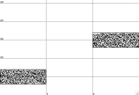
(draw (seq (note) (pause 1) (note :pitch 62)))
draw draws a piano roll representation of a musical object on the screen, as you can see in, e.g., Figure 1.
Figure 1:
The center of the notes height indicates the pitch and the
height itself indicates that amplitude. As you can see, the pitch and
the amplitude of both notes remain constant throughout the notes
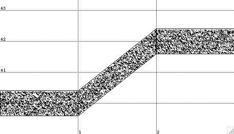
duration. Now we will put a note in between of these notes which
represents a glissando from the first to the second note. A glissando's
pitch glides linearly from the pitch of the first note to the pitch of
the second note. You see that we need a construct that enables us to
change an aspect of a note throughout its duration. This is what we
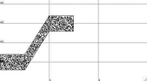
call a GTF, a generalized time function. Now we will give the code with a glissando instead of a pause (see Figure 2):
You can read (note :pitch (glissando 60 62)) as: a note
that has a line from 60 to 62 spread over its duration as a pitch. This
means that, if you will change the notes duration, the glissando will
adapt to the new duration and it will still be a glissando from 60 to
62. To demonstrate this, we will shrink the whole musical object (see
Figure 3).
Apparently, the glissando behaves well under transformation, since this
is how we intend a transformed glissando to behave. A different
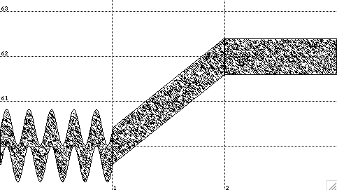
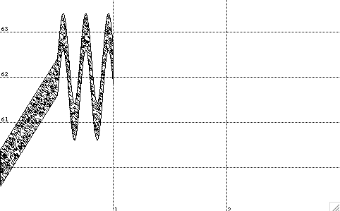
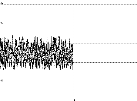
transformational behavior is shown in the vibrato example. Suppose we
want to add a nice vibrato to the first note. We can do that as follows
(also see Figure 4):
It might be self-explanatory that the keyword around indicates around which pitch the periodic deviation moves. The amplitude indicates how much the deviation from the notes pitch will be (vibrato has got more keywords which you can check out in the source code).
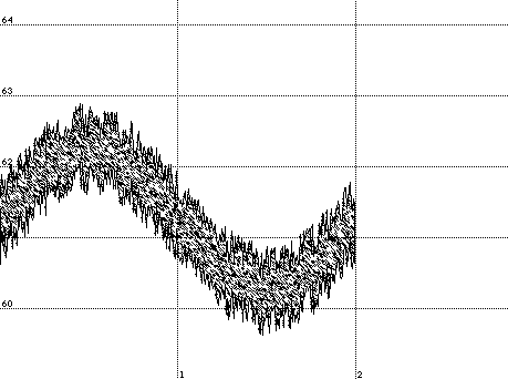
When we shrink this object, we want the vibrato of the first note not
to shrink. Instead we want the amount of periods to decrease. If the
vibrato would shrink the note would sound totally different and not the
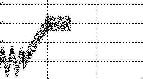
way we intend to. Now let us shrink the object again (see Figure 5):
As you can see, vibrato wonderfully behaves under this transformation like we intend to. To
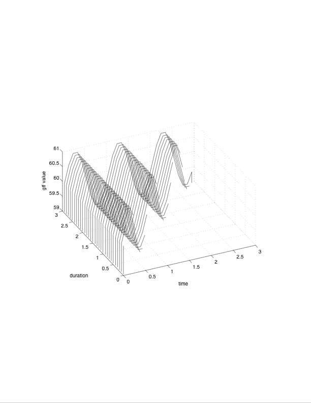
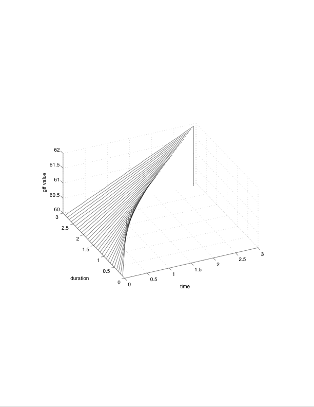
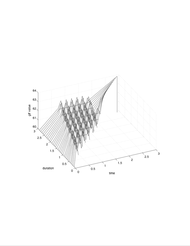
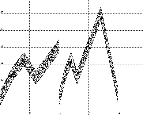
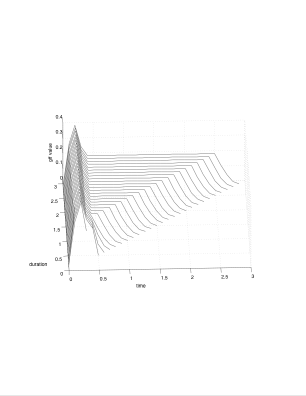
conclude this subsection we will give a 3D plot in which you can see
the behavior of a vibrato and a glissando within all possible durations
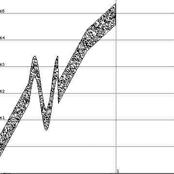
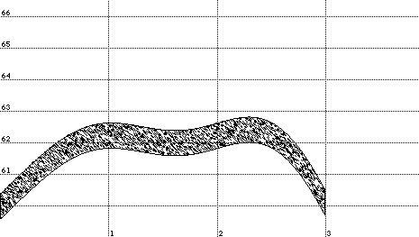
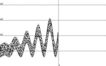
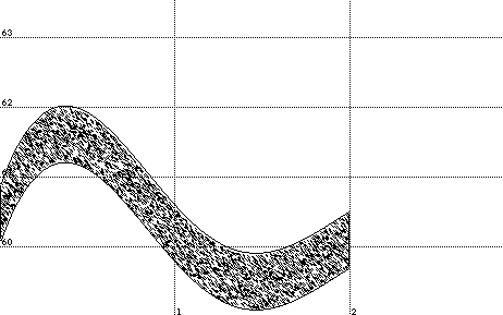
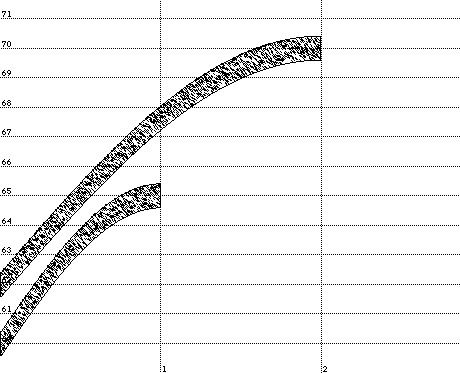
from the interval [0,3]. In Figure 6 ~\ref{fig:vibratograph} you see how the vibrato behaves in time for all durations. The NoteFun code for the vibrato is (vibrato :period 1).
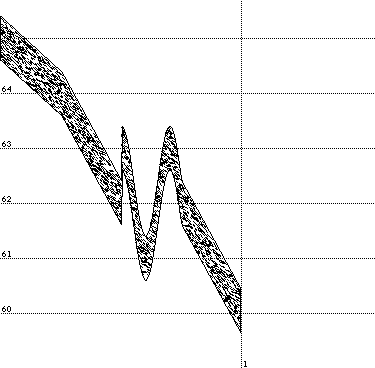
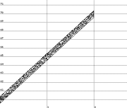
In Figure 7 ~\ref{fig:glissandograph} you see that the glissando goes
from 60 to 62 in a linear way according to the durations. The NoteFun code for the glissando is (glissando 60 62).
Figure 6:
Figure 7:
In the next section we will introduce four methods of creating new GTFs.
Creation of GTFs out of other GTFs
Creation of GTFs out of mathematical functions (lifting)
Creation of GTFs out of numeric tables
Creation of GTFs by writing your own Lisp code
Complex GTFs: creating GTFs out of other GTFs
Now we will introduce tools with which you can make complex GTFs from simpler ones. One is called concat-gtf
and like its name says, you can concatenate GTFs with it. With the ones
we already saw we can e.g., make a concatenation of a vibrato and a
glissando and apply it to one notes pitch. We will have to specify what
portion of a duration will be dedicated to what GTF. This is done by
means of absolute, relative and proportional who all indicate a point in time within the duration of a note in their own way. The argument list of concat-gtf is built up from alternating GTFs and indications of time.
An example of the use is given here (also see Figure 8):
You might wonder what (proportional .5) stands for.
It means that what is before this expression may take half (hence .5)
of the duration of the musical object, in this case a note, and what is
after this expression may take the other half. This means that (glissando 60 62) in this case may take up half a second, since the default duration of a note is 1 second, and (vibrato :around 62 :period .2) may take the rest which is also half a second.
If we transform the note by means of stretch
the durations of the GTFs will transform proportionally with the new
duration. Instead of proportionally determined points in time you can
also use relative points and absolute points.
Relative means in this case: seen from the start of the note. Absolute
means: seen from the start of the whole piece. Let us give a complex
example to demonstrate how relative and absolute behave under transformation (also see Figure 9):
You see this quite a complex beast. In this example there are two notes
in a sequence. The first has a duration of 4 seconds and the second has
a duration of 5 seconds. You can see that (proportional .25) (on line 3 and 11 of the above code fragment) indicate different points counted from the starts of the notes, as it stands for 4 x .25(=1) in the first note and 5 x .25(= 1.25) in the second note. The expression (relative 1.8)
indicates the same point in time counted from the starts of the notes,
namely 1.8 seconds after the start. This always holds, even when a note
has been transformed. The expression (absolute 3.5) indicates
the point in time that is 3.5 seconds after the start of the entire
musical object, in this case a sequence holding the two notes. (absolute 7.5) of course indicates the point in time 7.5 seconds after the start of the entire musical object. To hear the sound produced in this last example, click here:
Now answer these questions for yourself before trying out the encoding of the problems in NoteFun:
How will the musical object look when you add a (pause .5) in the sequence in front of the notes?
What will happen when you change the duration of the last note from 5 to 4?
In both cases, first try to calculate the new points in time where one GTF ends and another begins. Let us call those points switch points from now on. Afterwards look at the corresponding pictures and see if your guess was correct.
Now for a malicious use of concat-gtf, have a look at what happens here (also see Figure 10):
The glissando on line 3 takes half the note, as you can expect. But
what must be the behavior of the glissando on line 5, since the point
in time indicates by line 6 is before the point in time indicated by
line 4... ?
concat-gtf prints a warning on the screen saying: "Times being re-arranged!'' concat-gtf
checks if the successive switch points of its argument list are
monotonously increasing. Also it check whether all the switch points
remain between the bounds of the start and end time of the note. If
not, it changes the switch points so they will obey these two
properties.
In our last example concat-gtf changes the switch point on line 6 into (absolute .5) (first property) and the switch point on line 8 into (absolute 1)
(second property). The result is that the glissando of line 5 will not
appear since it has a time interval of exactly 0 seconds. The glissando
of line 5 will appear on the interval [.5,1]. The glissando
of line 9 will not appear since it has a time interval of 0 seconds. In
other words, the last example is equivalent to the following code:
Try this out and see for your self.
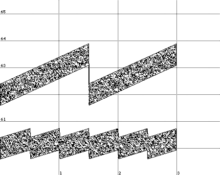
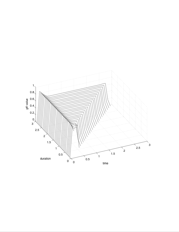
We conclude this subsection with a 3D graph of a complex GTF with duration from the interval [0,3] plotted in time. See Figure 11. The NoteFun code for this GTF is:
Note that until now we have only used GTFs in combination with the pitch of a note.
To stimulate your creativity we must remark that GTFs can also be used
in combination with a lot of other possible features of the note like amplitude and midi related parameters like brightness and pan.
To simulate a fade-out you can use a GTF that goes from 1 to 0, where 1
indicates full volume and 0 indicates total silence (also see Figure
12):
(draw (note :amplitude (ramp 1 0)))
Figure 12:
To hear the sound produced in this last example, click here:
As you might guess ramp is similar to
glissando. In fact, it is actually the same function. It only has a
more general name and unlike glissando its name will inspire us to use
it for all kinds of things, like here for amplitude.
To make use of the midi controller related features of note, you can add the synthesizer specific controller number and the range in which you want to control it yourself.
The code for the controllers that we have put in for our own synthesizer (A Yamaha MU90R) looks like this:
You can make up any keyword your want for your specific controller. The syntax for add-midi-controller is
(add-midi-controllers
	<keyword>
	<midi control number>
	<minimal-value>
	<default-value>
	<maximum-value>)
For a panning from left to right within a note we could write:
(note :pan (ramp -1 1))
You can remove a midi controller by executing (remove-midi-controller ). For example, if we want to remove the controller for brightness, we write: (remove-midi-controller :brightness). To get a list of all currently available midi controllers you write: (show-midi-controllers).
Complex GTFs continued
Another tool for merging simple GTFs into a complex one is switch-gtf. It works slightly different than concat-gtf
but has the same way of calling. Instead of concatenating GTFs it
switches between GTFs at certain switch points and the GTFs are all
spanned over the notes entire duration.
Let us give an example based on two glissando's, one going up and one
going down. Within the note we will switch between them using switch-gtf (also see Figure 13):
To hear the sound produced in this last example, click here:
switch-gtf corrects badly successive switch points in the same way as concat-gtf does.
Another way of building new GTFs from other ones is called time warping.
Instead of going through a GTF from left to right in time, we can e.g.,
do it from right to left; from the beginning to the end. This operation
can be done with a time warp that we called time-reverse. Its use is illustrated in the following example.
First we make a reference to a GTF to be able to write more readable code. We use the name some-gtf as the reference name. Then we draw the result of using some-gtf as a notes pitch (see Figure 14). Lastly we draw the result of a transformed version of some-gtf by means of the time warp time-reverse (see Figure 15).
Figure 14
Figure 15
To hear the sound produced in example illustrated by Figure 14, click here:
To hear the sound produced in example illustrated by Figure 15, click here:
Another handy time warp is make-time-cyclic. make-time-cyclic has one argument indicating a point time within the duration of the note by means of absolute, relative and proportional. I will show the use of make-time-cyclic by means of an example (see Figure 16):
Note that we have to set an other channel for either one of the notes, to make the example sound correctly.
To hear the sound produced in this last example, click here:
By now it might be clear how make-time-cyclic works.
The point in time indicated by the time switch is the period length
which indicates after what amount of time the GTF should start over
again as if it were from the start.
There are more facilities that let us create GTFs out of other ones. One is called mix-gtf. By means of an example we will show its use (see Figure 17):
The syntax in which you can use mix-gtf is:
(mix-gtf [<gtf> <factor>]*). The factors in this
expression can be real numbers or GTFs (the notation we have used for
the argument list must be read as a regular expression in which <gtf> and <factor>
can be arbitrary GTFs and numbers. The same holds for successive
examples in which this notation is used.). The result of this
expression will be a gtf which is the weighted result of the succeeding
gtfs and factors in the argument list. Our last example will be a gtf
which is the addition of a glissando from 60 to 70 and a sine with an
amplitude of 1 and a period of 2 seconds. Check Figure 18 and see if it
looks like you expect. Because of the fact that we can either fill in a
real number or a GTF as the factor, we are able to express things like:
"let the impact of a GTF run from 2 to 0 along with the duration of the
note". As follows:
The first GTF is kept constant (the succesive factor is 1) but
the second GTF is multiplied by a ramp from 2 to 0. What we will expect
is a ramp with a periodic deviation of which the amplitude will
decrease as we go through the note in time. You can see the result in
Figure 18.
Figure 18
Another similar combinator of GTFs is interpolate-gtf.
As its name suggests, it interpolates between two GTFs. To make this
clear let us interpolate between a glissando and a vibrato:
To give more elementary operations on GTFs we will introduce gtf+ and gtf*. After that we will introduce a more general function with which you can make your own operation on GTFs.
A GTF that is the sum of multiple other GTFs can be made with gtf+ with the following syntax:
(gtf+ [<gtf | number>]*). For example, we can add a
glissando and another glissando so that they will compensate each
other, resulting in a constant pitch:
The result is a note with a with-time-increasing periodic deviation from pitch 60 (see Figure 20).
If you require more operators on GTFs you can define them yourself using time-fun-compose. For example, if we would like to make the operator for division on GTFs we write:
(time-fun-compose #'/ [<gtf>]*)
More close to Lisp, a usable definition could be called gtf/ and would look like this:
In this section we will
describe how one can build a GTF based on a mathematical function, like
the sine function. This way of building gives one more degree of
freedom of customizing your own GTFs as you will not be only limited to
the tools we provided before. Instead you can come up with any unary
function, provided that they give a sensible result, you wish. We will
denote these functions with simple functions in what follows. You can
specify how it should behave under transformation. Like we saw with the
glissando, some functions should transform in a proportionally
stretching way. Other functions, similar to the vibrato, should not be
stretched. We call the creation of a GTF out of a simple function lifting.
An equivalent of the glissando might be a linear function, like (lambda(x) x).
Suppose
we want to have a simple function that corresponds to a glissando from
60 to 70. Note that we do not know the duration of the note, to which
the function will be applied, since it can be any positive real number.
For now we will just choose a function that goes from 60 to 70 in an
interval of 1 second:
(setq linfunc #'(lambda(x) (+ 60 (* 10 x))))
Now look at the following example (see Figure 22):
What does (lift linfunc (proportional-lift 0 1)) mean? Informally it means, select the function linfunc on the interval [0,1 and stretch it according to the duration of a note.
More general, the syntax for lift is:
(lift <lift-function>).
proportional-lift is a lift function that selects an interval
out of a simple function. Try to modify the duration of the note in the
last example and see that its pitch still runs from 60 to 70. This is
how we want a glissando to behave under transformation.
Another lift function is relative-lift.
It does not help us to stretch a selection out of a function but it
lets us express something else. Let us try it out as a variation on our
last example.
The behavior as result of this GTF is not the one we intend for a
glissando, as you can see in Figure~\ref{fig:lift-relative-1}. But
maybe you see where we \emph{do} want to go with our example, because
this is the kind of behavior we want to assign to a sine function to
make it behave like a vibrato, for example. The arguments of relative-lift
do not indicate an interval, but a starting point and an x-scale. This
makes it easy to create a nice vibrato out of a sine. Like this (see
Figure~\ref{fig:lift-relative-2}):
Now try to modify the duration of the note from the last
example again and see what happens! Is it the behavior you desire from
a vibrato?
The last lift function for simple functions we will discuss is absolute-lift. It is different from relative-lift in that it does not see the notes start as the starting point ( time = 0 )
for the GTF, but it uses the start of the whole musical object as the
starting point of the GTF. Let us illustrate this with a vibrato that
is lifted using absolute-lift and that is used over a group of notes.
Because the starting point of the whole group of notes is taken as time = 0
you can see the sine wave continuously running through all notes, as if
it does not know where one note ends and another begins.
Lifting tables
Another method of creating GTFs is by means of tables. You can specify
a table with key and value pairs and lift it as if it were a
mathematical function. An example is given below.
With the help of table-fun we can make a simple function out of a table:
(setq tablefunction (table-fun my-table))
Since tablefunction now is a simple function, we
can use it in the same way as any other simple function. Hence we can
lift it with the same constructions as demonstrated in the previous
subsection. The function is made by a lineair interpolation between the
values of the table, as demonstrated in the following code (see Figure
25):
In this last
subsection on the creation of GTFs we will address you to write your
own Lisp code as a means of creating your own GTFs. In order to do that
we have to go into details of how a GTF is built up.
We will do this, like you are used to in this tutorial, by means of
example. First we will show how an existing GTF is built up. After that
we will write a new one from scratch.
Do you remember the glissando GTF from all the previous examples? As we already said it is the same function as the ramp function. Here is its encoding in Lisp:
1(defun ramp (from to)
2 (gtf (start duration)
3    (tf(time)
4      (let ((progress (/ (- time start) duration)))
5        (+ from (* progress (- to from)))))))
In general a GTF is built up using the construction
(gtf (start duration)
  (...
   (tf (time) (...))...)
ramp returns a function of the type R -> R+ -> (R+ -> R+).
The constructions gtf and tf work like normal functional abstraction. They are adapted versions of Lisps lambda, enhanced for our purpose here. gtf creates a function of the type R+ -> R+ -> (R+ -> R+) and tf creates a funtion of type R+ -> R+.
A GTF makes use of three important variables time, start and duration. The variable time indicates the time counted from the start of an entire musical object; start indicates the time at which the note in which the GTF will be used will begin; duration represents the time interval on which a note will be played.
The dots on the second line of the general code are intended to consist of calculations with start and duration. Calculations that involve also time can only occur inside the tf
construction. This two layer way of building a GTF is chosen because of
efficiency reasons which we will not have to discuss on this website
(look at my internship report for more on this). Because all of the
calculations that we need in ramp involve time, they have to occur inside the tf.
Now let us look how ramp works. On line 4 of its code an expression with time, start and duration is bound to progress.
If we look closer to the expression we see that it indicates the
fraction of the duration that has already passed: "current time minus
start time" divided by "total duration of the note". At the very start
of the note, progress will have value 0. At the very end of the note "time minus start" will equal duration and therefore progress will have the value of 1. Now, with (ramp ) we want to have a GTF that is a linear function from to on the interval [start,start+duration]. Note that the expression (+ from (* progress (- to from))))))) returns the right value on each point of time on in the interval.
Now that we have seen the implementation of ramp it may inspire us to make a different GTF.
Wouldn't it be funny to make a GTF that gives random values from a certain range? In Lisp (random ) returns a random floating point number from the range [0,n[ (n self is excluded) when n is a floating point number. Hence (random 1.0) returns a floating point number between 0 and 1. The Lisp expression (+ min (* (- max min) (random 1.0))) then returns a random value between min and max. This is all we have to return, so the code for random-gtf will be quite simple:
(defun random-gtf (min max)
  (gtf (start duration)
    (tf (time)
      (+ min (* (- max min) (random 1.0))))))
Let us see how random-gtf behaves as a pitch GTF:
(play-and-draw (note :pitch (random-gtf 61 62)))
Look at Figure 26 for the result!
Figure 26
To hear the sound illustrated by Figure 26, click here:
Of course we can also use random-gtf to make small random deviations from other GTFs like in the following example (see Figure 27):
To hear the sound illustrated by Figure 27, click here:
Case study: ADSR
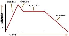
To conclude this tutorial, we will give you a description of how to
build a GTF that behaves like an instrument. This GTF will be build up
in analogy of a concept in the synthesizer world, namely ADSR. ADSR
stands for attack, decay, sustain and release. The idea is that when a note starts, the volume of the note will go from 0
to a certain attack level. Immediately after reaching the attack level
the volume will go down in a certain amount of time, till it reaches
the sustain level. This level will be maintained for a certain length
of time. Just before the end of the note (think of a key being
released) the level will go from sustain level to 0 again.
This is illustrated in Figure 28. We will discuss a simplified version
of this idea for the sake of didactics and the length of this tutorial.
Figure 28
From the above description of ADSR it might be evident that we need four basic GTFs which we can concatenate later by means of concat-gtf. Conceptually this may look something like this:
1(concat-gtf
2 attack function
3 time switch
4 decay function
5 time switch
6 sustain function
7 time switch
8 release function)
We need a GTF for going from 0 to an attack level in
a certain amount of time. This amount of time does not in- or decrease
with the length of a note for most instruments (loosely speaking); it
is a constant portion of time. Therefore, the attack function, let us
call it attack-fun, must precede a time switch that is made with relative. The same goes for the decay function, which we will call decay-fun and its succeeding time switch. The sustain, named sustain-fun, does depend on the duration of the note. The portion of time needed for the release, let us call it release-fun, from sustain level to 0 is again a constant portion. With this information we can make the concept a bit more concrete:
The expression (fun-funcall #'- #'end-time release-time) evaluates to the end time of the note minus the time interval indicated by release-time. Because end-time and release-tim are not normal numbers (actually they are functions) we have to use fun-funcall in this case.
Now let us try out adsr. We define two different ADSRs named inst1 and inst2 as follows and use both in a group of notes:
You see that the only the length of the sustain phases
depend on the lengths of the notes. The other phases are of constant
length, no matter what the lengths of the notes are.
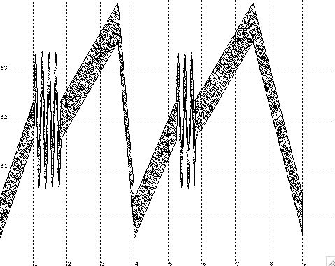
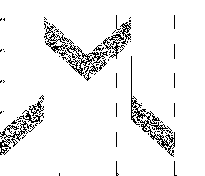
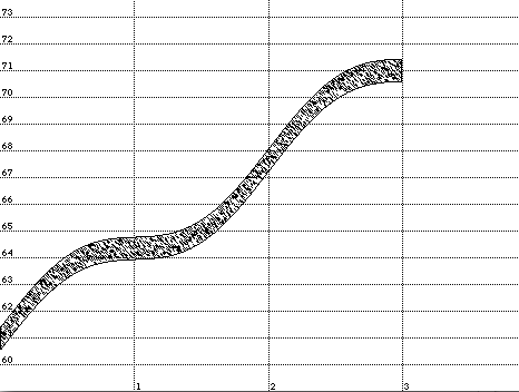
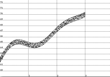
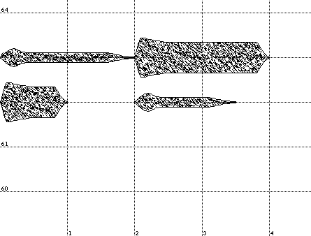
In the following graphs we show both ADSRs plotted in time against durations of lenghts from the interval [0,3] in seconds.
Figures 32 (left) and 33 (right)
Some additional notes
All the sounds were recorded using a Yamaha MU90R synthesizer.
If you find any mistakes on this page, please report them to me. Also other comments are welcome at michielborkent@gmail.com.